Scaling bioremediation isn’t simply a matter of enlarging a successful lab test. Laboratory treatment uses small volumes measured in litres or kilograms; pilot plots can involve hundreds of kilograms or hundreds of cubic metres, while full-scale projects may cover hectares of soil or kilometres of coastline. The right scale depends on whether treatment conditions can be reproduced across the site, including at the target depth.

A promising bench result is therefore a starting point, not a complete field design. Soil structure, contaminant distribution, and access to oxygen or nutrients can all affect biological treatment below ground.

This article explains how laboratory, pilot, and full-scale approaches differ, and how depth should inform treatment decisions. It also explores enzymes and in situ treatment, including why delivery and contact with contaminants matter as conditions change through the soil profile.

Each scale answers a different engineering question: can the treatment work, how does it perform under site conditions, and how can it be applied across a larger area? This practical framework helps match bioremediation to the site instead of assuming one treatment design will suit every depth.

In situ remediation of petroleum hydrocarbons

In situ treatment stimulates biological activity where petroleum hydrocarbons remain, including in soil and groundwater. Its performance depends on where contaminants are located, subsurface conditions, and whether treatment reaches the contaminated zone.

In Situ and Ex Situ Methods

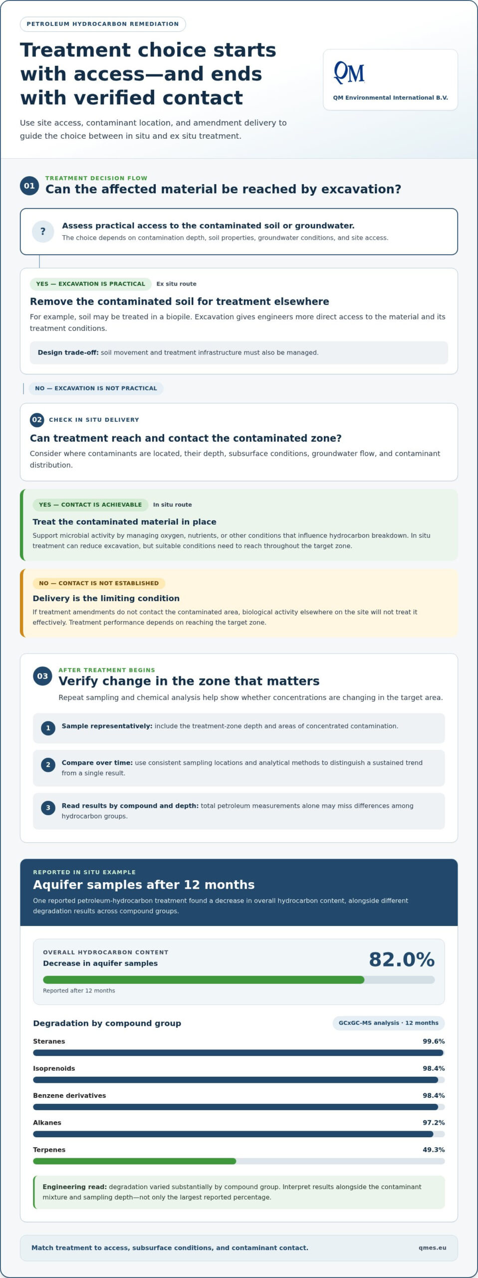
In situ bioremediation treats contaminated soil or groundwater without excavating the affected material. Engineers may support microbial activity by managing oxygen, nutrients, or other conditions that influence hydrocarbon breakdown. This approach can reduce excavation, but treatment depends on delivering suitable conditions throughout the target zone.

Ex situ treatment involves removing contaminated soil for treatment elsewhere, such as in a biopile. Excavation gives engineers more direct access to the material and its treatment conditions, but also changes how soil movement and treatment infrastructure are managed. The choice depends on contamination depth, soil properties, groundwater conditions, and site access.

For petroleum hydrocarbons below ground, in situ treatment is relevant when excavation cannot practically reach the affected aquifer. Field design must account for groundwater flow and contaminant distribution. If treatment amendments do not contact the contaminated area, biological activity elsewhere on the site will not treat it effectively.

Verifying Remediation Outcomes

Repeat sampling and chemical analysis help verify whether contaminant concentrations are changing in the target area. Sampling locations should represent the treatment zone, including its depth and areas of concentrated contamination. Comparing results over time helps distinguish a sustained trend from a single sample result.

One reported in situ petroleum-hydrocarbon treatment found an 82.0% decrease in hydrocarbon content in aquifer samples after 12 months. GCxGC-MS analysis after 12 months found degradation of 99.6% for steranes, 98.4% for isoprenoids, 98.4% for benzene derivatives, 97.2% for alkanes, and 49.3% for terpenes. The different results show why total petroleum measurements alone can miss differences among compound groups.

Engineers can compare baseline and follow-up samples using consistent analytical methods and locations. For example, GCxGC-MS can help characterize changes in specific hydrocarbon groups, while aquifer sampling tracks overall content. Interpretation should account for the contaminant mixture and sampling depth, not just the largest reported percentage.

Large-Scale Case Studies

Before describing a specific project as a large-scale success, identify its site, contaminant, treatment footprint, and monitoring results. The quantified aquifer example above reports treatment outcomes but does not identify a U.S. site. Its percentages therefore cannot support a claim about a named U.S. case study.

For an engineering comparison, a useful case record separates treatment scale from treatment performance. It identifies whether contamination was treated in place, reports the sample medium, and shows how results changed over time. The 12-month aquifer measurements illustrate why contaminant-specific analysis matters: terpenes and steranes showed markedly different degradation results.

Apply the same evidence standard when assessing a U.S. project: connect the treatment area to sampling locations, then compare contaminant results across monitoring events. A reported decrease matters only in relation to the compounds measured and the portion of the site sampled. This distinction keeps project comparisons technically grounded.

Defining laboratory, pilot, and full-scale bioremediation

Scale describes the amount of contaminated material treated and the conditions a project must manage. Laboratory, pilot, and full-scale work answer different questions before treatment reaches its intended footprint.

Laboratory, Pilot, and Full-Scale Definitions

Laboratory-scale bioremediation tests treatment in small volumes measured in litres or kilograms. This controlled setting helps compare conditions and determine whether biological treatment affects the target contaminant. It cannot represent every field condition: soil structure, contaminant distribution, and delivery constraints can vary across a site.

Pilot-scale bioremediation tests treatment under more representative conditions, using plots involving hundreds of kilograms or hundreds of cubic metres of material. The larger volume helps engineers evaluate performance beyond a laboratory vessel. A pilot can reveal practical issues with amendment delivery, treatment coverage, or variation across the zone.

Full-scale bioremediation applies treatment across the project footprint, which may cover hectares of soil or kilometres of coastline. Scale is defined by the area and material requiring treatment, not simply by using more of a laboratory formulation. Field design must account for site layout, access, and spatial differences in contamination.

These stages form a progression, but they are not interchangeable. Laboratory results establish treatment response under controlled conditions. Pilot work tests how well that response transfers to a representative area. Together, the phases provide a controlled basis for scaling bioremediation, with each informing the next. A bench test may show biological activity, for example, while a pilot reveals whether treatment reaches soil evenly.

Scale selection connects evidence to design decisions. Small samples help compare treatment conditions, while larger plots reveal operational constraints. At full scale, contaminant mapping and sampling design become central to interpretation. For scaling bioremediation beyond a pilot, engineers can use Site Assessment and Remediation Planning to organize site conditions, test results, and field objectives into a treatment strategy.

Timelines at Pilot and Full Scale

Pilot and full-scale timelines depend on the contaminant, soil conditions, treatment method, and monitoring objectives. Project duration cannot be inferred from area alone. Biological activity, contaminant accessibility, and the ability to maintain suitable treatment conditions all affect how quickly concentrations change.

A reported China biopiling treatment of PAH-contaminated soil reduced benzo[a]pyrene from 1.50 mg/kg to 0.51 mg/kg in seven days. This is a measured result for a specific contaminant and setup, not a standard duration for other pilot projects or full-scale sites.

Use pilot monitoring to assess the rate and consistency of change under site-relevant conditions. Compare samples from corresponding treatment areas and consider whether measured compounds respond at similar rates. If performance varies across a plot, the full-scale schedule and treatment layout may need adjustment.

At full scale, duration also reflects the project footprint and the sampling required to evaluate it. Treatment may progress unevenly where soil conditions or contaminant concentrations vary. A practical schedule links treatment phases to measured performance instead of assuming a pilot’s calendar will apply to a larger site.

Depth-specific degradation rates

Hydrocarbon degradation can vary with depth, so a site-wide rate may conceal meaningful differences. An exponential decay model estimated the greatest hydrocarbon decomposition rate at 8-10 m in an aquifer. At that depth, the average hydrocarbon decay constant was 0.227. These values describe a depth-specific model result, not a universal rate for every aquifer or contaminant. Keeping the result tied to its depth helps engineers interpret what the estimate actually represents.

Subsurface conditions shape contact between microbes, contaminants, and resources that support biological activity. Soil texture, groundwater movement, and oxygen availability can differ between shallow and deeper zones. Those conditions influence contaminant movement and treatment access. Surface samples alone may not show how deeper material responds. For example, the 8-10 m interval could have different conditions from soil nearer the surface, so separate depth records matter.

Organize characterization and monitoring by defined depth intervals. First, map the vertical distribution of hydrocarbons using samples collected at specified depths. Then compare concentrations within matching intervals over time. Measurements from 8-10 m should be assessed separately from shallow-soil results. This comparison helps distinguish depth-related treatment response from changes caused by different sampling locations or contaminant mixtures. Consistent intervals also make field observations easier to compare.

The decay constant of 0.227 needs its model context for interpretation. A decay constant is a parameter in an exponential model describing change. By itself, it does not state a percentage removed or a duration. Its time basis and application conditions matter. During scaling bioremediation, engineers should keep the value paired with the reported depth, aquifer setting, and model, rather than converting it into an unsupported cleanup timeline.

Depth-resolved findings can guide where treatment and monitoring focus. If results show slower change in one interval, engineers can examine whether treatment reaches that zone and whether local conditions support biodegradation. If the 8-10 m interval shows a greater modeled rate, that finding can inform design comparisons and sampling priorities. It should not justify overlooking other depths, where contaminant concentrations and treatment responses may differ.

For larger-scale design, link each rate estimate to its sample depth, contaminant measurement, and analytical model. Compare equivalent intervals across monitoring events, then assess whether observed trends align with the model. This helps translate depth-specific evidence into treatment placement and monitoring decisions. Scaling bioremediation with depth-resolved data keeps estimates relevant to the sampled aquifer, rather than applying one interval’s results across the entire remediation footprint.

What is bioremediation and how does it work?

Bioremediation uses microorganisms or their enzymes to transform contaminants in soil, sediment, or groundwater. In oil-impacted soil, for example, microbial communities can use petroleum hydrocarbons as substrates during metabolism. This biological activity changes contaminant molecules through biochemical reactions. Treatment design considers the organisms, enzymes, and site conditions that support these reactions, as well as where contaminants are located and whether biological activity can reach them.

Microorganisms obtain energy and materials through metabolism, a set of reactions that can alter contaminants. Some organisms already present in the environment carry out these reactions; other approaches add selected microorganisms or enzymes to support a treatment objective. Enzymes act as biological catalysts: they help reactions occur but are not living cells themselves. Their activity depends on contact with the target compound and suitable surrounding conditions.

For petroleum hydrocarbons, biological reactions can transform compounds into smaller products and, through further reactions, into carbon dioxide, water, and microbial biomass. The pathway depends on the contaminant’s molecular structure. A complex hydrocarbon mixture, for example, contains compounds that microbial communities may process differently. Measuring only total petroleum content may therefore miss how individual compounds respond. Chemical analysis can distinguish overall change from changes in specific contaminant groups.

Oxygen availability influences microbial pathways. In oxygen-rich settings, aerobic organisms use oxygen in metabolism; other organisms can function through different pathways when oxygen is limited. Nutrient availability, moisture, temperature, pH, and contaminant accessibility also shape biological activity, and these factors interact. Microbes cannot transform hydrocarbons that remain physically inaccessible, even when other conditions support their activity.

Enzymes can participate directly in contaminant transformation, and microorganisms can produce enzymes as part of their metabolism. Either way, treatment depends on delivery and contact. An enzyme applied to soil must reach the contaminant, and the local environment must support its activity. In groundwater, flow paths affect how treatment materials move through the aquifer. Site characterization helps identify conditions that influence placement and contact.

Bioremediation can treat contamination in place, including in soil, sediment, or groundwater, or treat excavated material elsewhere. The choice affects how engineers manage access, treatment conditions, and monitoring. In situ treatment avoids moving contaminated soil but requires effective contact underground. Ex situ treatment allows direct handling of excavated material. In either case, sampling and chemical analysis track contaminant changes and help assess whether treatment is working as designed.

How long does bioremediation take at pilot and full scale?

No single duration applies to every pilot or full-scale project. Treatment time depends on the contaminant, its accessibility, subsurface conditions, and how quickly biological activity changes concentrations. A useful schedule ties treatment phases to monitoring results instead of assuming a small test predicts the timeline for a large site.

A reported China biopiling treatment of PAH-contaminated soil reduced benzo[a]pyrene by 66% in seven days. This result gives a concrete example of change measured during a defined treatment period. It doesn’t establish a standard seven-day treatment duration: contaminant mixtures, soil conditions, and treatment setups differ between sites.

At pilot scale, engineers use monitoring to determine whether treatment is progressing under representative conditions. The schedule should account for when samples are collected, how concentrations are measured, and whether results show a consistent trend. A change in one sample, for example, may not represent the entire test plot. Comparing results from corresponding locations helps show whether treatment is uniform or uneven.

Full-scale work adds the site footprint to the timing decision. A project covering hectares of soil or kilometres of coastline involves spatial variation that a pilot plot may not capture. Sampling must represent the treatment area, and access to different zones can affect monitoring logistics. Treatment may need to continue in one zone while another responds differently.

Engineers can make schedules more useful by linking each phase to a measurable question: Is the target contaminant changing? Does the trend hold across sampling locations? Are some parts of the treatment area responding differently? These comparisons help determine whether to continue the current approach, adjust treatment conditions, or revise the monitoring plan. The measured endpoint matters as much as elapsed time.

Enzyme and microbial activity, along with contaminant availability, influence the observed pace. Hydrocarbons that are difficult to reach may respond differently from compounds in direct contact with treatment. At pilot scale, this difference can inform full-scale monitoring and treatment placement. At full scale, the sampling plan should preserve information about depth and distribution instead of averaging it into one site-wide result.

For a schedule grounded in site conditions, Site Assessment and Remediation Planning can connect pilot findings, sampling design, and full-scale treatment decisions. Define measurable endpoints, compare results across treatment zones, then use those trends to guide the next project phase.

QM Environmental International B.V.: MicroCat-XBS

QM Environmental International B.V. offers MicroCat-XBS as part of its environmental management portfolio. For engineers evaluating biological treatment, these offerings can be considered against site conditions, contaminant distribution, and treatment objectives. Product selection should reflect the project’s technical requirements, not scale alone.

QM Environmental International B.V. also offers multiple products for aerobic bioremediation such as nutrients like MicroCat-NPN, MicroCat-NPC and MicroCat-SH (wetting agent). These products can be considered alongside MicroCat-XBS when planning a site-specific approach. Site assessment and remediation planning help connect treatment decisions with relevant conditions, including soil depth and the intended treatment footprint. EOx, an oxygen release compound can be used to stimulate the aerobic degradation.

To discuss your bioremediation project, contact QM Environmental International B.V. or visit qmes.eu.

Turn site data into a treatment plan

The next step in scaling bioremediation is to connect site characterization with a treatment design that reflects contaminant distribution, soil depth, and monitoring needs. Identify the questions that remain open before expanding treatment, then use site-specific evidence to guide decisions. Treatability studies can assess how a biological approach responds to a particular site’s conditions.

QM Environmental International B.V. offers MicroCat-XBS, NPN, NPC, SH, EOS organic substrates, BAC9, EOx, EAS, CoBUPHmg, and QM-ZviER (zero valent iron) as part of its environmental management portfolio. Consider these options alongside project assessment and remediation planning, tying treatment choices to site objectives rather than scale alone.

If you’re developing a bioremediation project, discuss the site conditions and treatment goals with QM Environmental International B.V. Contact QM Environmental International B.V to explore a practical next step for your project.

Frequently Asked Questions

What factors determine whether a bioremediation project can be scaled up successfully?

Successful scale-up depends on treatment reaching the contaminants and sustaining the biological conditions needed for degradation. Engineers assess the contaminant mixture, soil permeability, groundwater movement, nutrient and oxygen availability, and spatial variability across the site. A pilot that treats uniform soil may not transfer directly to a site with layered sediments or isolated hotspots. Sound scale-up decisions connect pilot performance to field conditions, treatment delivery, and representative monitoring locations.

What are the steps for scaling a laboratory bioremediation process to pilot and full scale?

Move from controlled testing to a representative pilot, then use the evidence to design full-scale application. First, test treatment conditions against the site’s contaminants and soil. Next, set up a pilot that reflects field materials and delivery constraints. Track treatment response and operational issues, then refine the design before expanding it. Uneven results across a pilot plot, for example, may prompt changes to amendment placement or sampling locations before full-scale work.

How much does large-scale bioremediation cost per cubic yard or gallon?

No single cost per cubic yard or gallon applies to every project. Price depends on contaminant type and concentration, soil or groundwater conditions, treatment method, site accessibility, treatment volume, and monitoring needs. In situ and excavated-soil approaches also involve different work and logistics. A project-specific estimate depends on the scope and site conditions and is provided after a quote request.

What monitoring methods and performance metrics are used to verify bioremediation at scale?

Use repeated sampling with consistent locations, depths, and laboratory methods to evaluate treatment performance. Track contaminant concentrations and, where relevant, specific compounds or transformation products. Field measurements such as dissolved oxygen, pH, and oxidation-reduction conditions can help explain why concentrations change or stall. Comparing monitoring wells along groundwater flow paths, for example, can show whether a treatment response is limited to one zone or extends through the affected area.

What are the risks and limitations of scaling bioremediation, including contaminant rebound and unintended byproducts?

Scale-up can reveal uneven treatment, limited amendment delivery, or site conditions that slow biological activity. Rebound can occur if contaminant mass remains in less accessible soil and later moves into groundwater or sampled areas. Microbial transformation can also produce intermediate compounds, so measuring only the original contaminant may miss important changes. A monitoring plan should track relevant parent compounds and transformation products, compare results across treatment zones, and continue monitoring after active treatment ends.

What EU regulations apply to large-scale bioremediation projects?

Applicable requirements depend on the EU country, site location, contaminants, affected media, cleanup program, and treatment activities.Environmental frameworks vary per EU member and may address cleanup decisions, groundwater or surface-water impacts, amendment placement, and excavated-material management. Build a regulatory review around the actual remedy: identify where treatment occurs, what enters the subsurface, and whether soil or water is moved or discharged. These project details determine which federal and state requirements apply.